Efficiency comes in two flavors:
- Programming Cost (not mention in this course)
- How long does it take for you to develop your programs?
- How easy is it to read or modify your code?
- How maintainable is your code? (very important — much of the cost comes from maintenance and scalability, not development.)
- Execution Cost
- Time complexity: How much time does it take for your program to execute?
- Space complexity: How much memory does your program require?
Example of Algorithm Cost
Objective: Determine if a sorted array contains any duplicates.
| -3 | -1 | 2 | 4 | 4 | 8 | 10 | 12 |
Silly Algorithm: Consider every pair, returning true if any match.
Better Algorithm: Take advantage of the sorted nature of our array.
Techniques for measuring computational cost:
Technique 1: Measure execution time in seconds using a client program.
Procedure:
- Use a physical stopwatch
- Or, Unix has a built in time command that measures execution time.
- Or, Princeton Standard library has a stopwatch class
Example in using stopwatch class of Princeton Standard library:
1
2
3
4
5
6
7
8
9
10
11
12
13
14
15
16
17
18
19
20
21
22
23
24
25
26
27
28
29
30
31
32
public class dup1 {
    //Silly Duplicate: compare everything

    public static boolean dup1(int[] A) {
        for (int i = 0; i < A.length; i += 1) {
            for (int j = i + 1; j < A.length; j += 1) {
                if (A[i] == A[j]) {
                    return true;
                }
            }
        }
        return false;
    }

    public static int[] makeArray(int N) {
        int[] A = new int[N];
        for (int i = 0; i < N; i++) {
            A[i] = i;
        }
        return A;
    }

    public static void main(String[] args) {

        int N = Integer.parseInt(args[0]);
        Stopwatch sw = new Stopwatch();
        int[] A = makeArray(N);
        dup1(A);
        double secondsElapsed = sw.elapsedTime();

        StdOut.println("Seconds elapsed = " + secondsElapsed);
    }
}
Output of dup1:

1
2
3
4
5
6
7
8
9
10
11
12
13
14
15
16
17
18
19
20
21
22
23
24
25
26
27
28
29
30
public class dup2 {
    //Better Duplicate: compare only neighbors

    public static boolean dup2(int[] A) {
        for (int i = 0; i < A.length - 1; i += 1) {
            if (A[i] == A[i + 1]) {
                return true;
            }
        }
        return false;
    }

    public static int[] makeArray(int N) {
        int[] A = new int[N];
        for (int i = 0; i < N; i++) {
            A[i] = i;
        }
        return A;
    }

    public static void main(String[] args) {
        int N = Integer.parseInt(args[0]);
        Stopwatch sw = new Stopwatch();
        int[] A = makeArray(N);
        dup2(A);
        double secondsElapsed = sw.elapsedTime();

        StdOut.println("Seconds elapsed = " + secondsElapsed);

    }
}
Output of dup2:

- Pros: Easy to measure, meaning is obvious.
- Cons: May require large amounts of computation time. Result varies with machine, compiler, input data, etc.
This method is simple, but not mathematically rigorous. The results may not clearly demonstrate the relationship between contrasts.
Technique 2A: Count possible operations for an array of size N = 10,000.
1
2
3
4
5
6
7
8
for (int i = 0; i < A.length; i += 1) {
    for (int j = i+1; j < A.length; j += 1) {
        if (A[i] == A[j]) {
            return true;
        }
    }
}
return false;
times of operation:
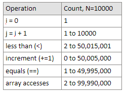
In the worst case: j = i + 1: when i=0 to i=9999, j=1 to j=10000. Number of assignment from 1 to 10000 equals to 10000.
less than (<):
- Outer layer for loop: from i=0 to i=10000, number of comparisons equals to 10001.
- Inner layer for loop: when i=0, j=1 to j=10000, j compares 10000 times; when i=9999, j=10000, j compares once. 1+2+…+10000 = 50005000.
- Total number of comparisons = 10001+50005000 = 50015001.
increment (+=1):
- Outer layer for loop: i increases from 0 to 10000, total increased number of times equals to 10000.
- Inner layer for loop: when i=0, j=1 to j=10000, j increases 9999 times; when i=9998, j=9999 to j=10000, j increases once. 1+2+…+9999 = 49995000.
- Total number of increments = 10000+49995000 = 50005000.
equals: In the worst case, each item has to be compared with the items after it. From i=0 to i=9998, number of equals = 9999 + 9998 + … + 1 = 49995000.
array accesses: Number of array accesses = 2 * equals = 2 * 49995000 = 99990000.
Procedure:
- Look at your code and the various operations that it uses (i.e. assignments, incrementations, etc.)
- Count the number of times each operation is performed.
Observations:
- Some counts get tricky to count.
- How did we get some of these numbers? It can be complicated and tedious.
Pros vs. Cons:
- Pros: Machine independent (for the most part). Input dependence captured in model.
- Cons: Tedious to compute. Array size was arbitrary (we counted for N = 10,000 — but what about for larger N? For a smaller N? How many counts for those?). Number of operations doesn’t tell you the actual time it takes for a certain operation to execute (some might be quicker to execute than others).
So maybe this one has solved some of our cons from the timing simulation above, but it has problems of its own.
Technique 2B: Count possible operations in terms of input array size N (symbolic counts)
Symbolic counts:
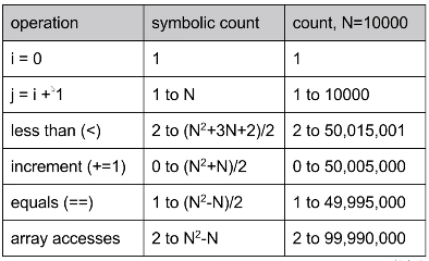
- Pros: Still machine independent (just counting the number of operations still). Input dependence still captured in model. But now, it tells us how our algorithm scales as a function of the size of our input.
- Cons: Even more tedious to compute. Still doesn’t tell us the actual time it takes.
Scaling Matters
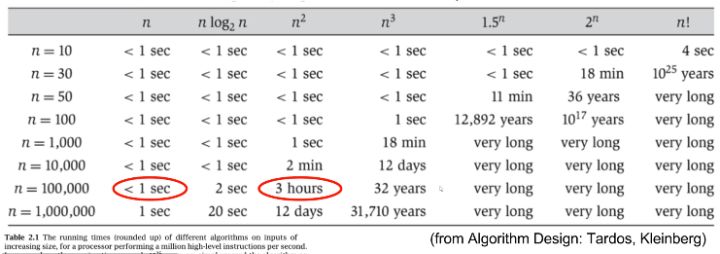
Asymptotic Behavior
In most cases, we only care about what happens for very large N. We want to consider what types of algorithms would best handle big amounts of data, such as in the examples listed below:
- Simulation of billions of interacting particles
- Social network with billions of users
- Encoding billions of bytes of video data
Simplification steps:
- Only consider the worst case.
- Pick a representative operation (aka: cost model)
- Ignore lower order terms
- Ignore multiplicative constants.
Summary of our (Painful) Analysis Process
- Construct a table of exact counts of all possible operations (takes lots of effort!)
- Convert table into worst case order of growth using 4 simplifications.
Simplified Analysis Process
Rather than building the entire table, we can instead:
- Choose our cost model (representative operation we want to count).
- Figure out the order of growth for the count of our representative operation by either:
- Making an exact count, and discarding unnecessary pieces
- Or, using intuition/inspection to determine orders of growth (comes with practice!)
Formalizing Order of Growth
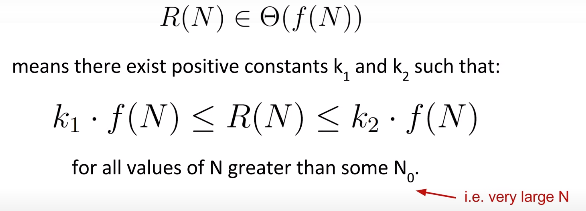
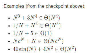
Big-Theta:
formal definition
Big O:
Whereas big theta can informally be thought of as something like ‘equals’, big O can be thought of as ‘less than or equal’.

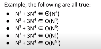
Big-theta 强调表达“等于”,一般用于对具体情况下runtime的描述,比如:The worst case runtime is Θ(N²) , the best case runtime is Θ(1) ,需要有一个明确的对situation的界定。
Big-O 强调表达“小于或等于”,不需要有具体的situation,比如:the runtime is O(N²) , 表达的是整体的runtime都小于或等于 N² 。
To summarize the usefulness of Big O:
- It allows us to make simple statements without case qualifications, in cases where the runtime is different for different inputs.
- Sometimes, for particularly tricky problems, we (the computer science community) don’t know the exact runtime, so we may only state an upper bound.
- It’s a lot easier to write proofs for Big O than Big Theta, like we saw in finding the runtime of merge-sort in the previous chapter. This is beyond the scope of this course.
Big-Omega:
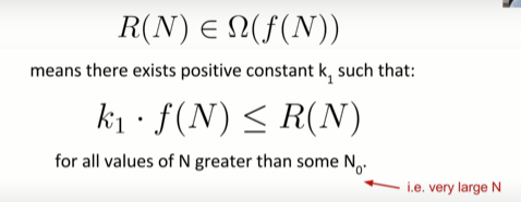
强调“大于或等于”
